Supervised Learning
Project: Finding Donors for CharityML
In this project, you will employ several supervised algorithms of your choice to accurately model individuals’ income using data collected from the 1994 U.S. Census. You will then choose the best candidate algorithm from preliminary results and further optimize this algorithm to best model the data. Your goal with this implementation is to construct a model that accurately predicts whether an individual makes more than $50,000.
This sort of task can arise in a non-profit setting, where organizations survive on donations. Understanding an individual’s income can help a non-profit better understand how large of a donation to request, or whether or not they should reach out to begin with. While it can be difficult to determine an individual’s general income bracket directly from public sources, we can (as we will see) infer this value from other publically available features.
The dataset for this project originates from the UCI Machine Learning Repository. The datset was donated by Ron Kohavi and Barry Becker, after being published in the article “Scaling Up the Accuracy of Naive-Bayes Classifiers: A Decision-Tree Hybrid”. You can find the article by Ron Kohavi online. The data we investigate here consists of small changes to the original dataset, such as removing the 'fnlwgt' feature and records with missing or ill-formatted entries.
Exploring the Data
Run the code cell below to load necessary Python libraries and load the census data. Note that the last column from this dataset, 'income', will be our target label (whether an individual makes more than, or at most, $50,000 annually). All other columns are features about each individual in the census database.
1 | # Import libraries necessary for this project |
| age | workclass | education_level | education-num | marital-status | occupation | relationship | race | sex | capital-gain | capital-loss | hours-per-week | native-country | income | |
|---|---|---|---|---|---|---|---|---|---|---|---|---|---|---|
| 0 | 39 | State-gov | Bachelors | 13.0 | Never-married | Adm-clerical | Not-in-family | White | Male | 2174.0 | 0.0 | 40.0 | United-States | <=50K |
Implementation: Data Exploration
A cursory investigation of the dataset will determine how many individuals fit into either group, and will tell us about the percentage of these individuals making more than $50,000. In the code cell below, you will need to compute the following:
- The total number of records,
'n_records' - The number of individuals making more than $50,000 annually,
'n_greater_50k'. - The number of individuals making at most $50,000 annually,
'n_at_most_50k'. - The percentage of individuals making more than $50,000 annually,
'greater_percent'.
** HINT: ** You may need to look at the table above to understand how the 'income' entries are formatted.
1 | # TODO: Total number of records |
Total number of records: 45222
Individuals making more than $50,000: 11208
Individuals making at most $50,000: 34014
Percentage of individuals making more than $50,000: 24.78439697492371%
** Featureset Exploration **
- age: continuous.
- workclass: Private, Self-emp-not-inc, Self-emp-inc, Federal-gov, Local-gov, State-gov, Without-pay, Never-worked.
- education: Bachelors, Some-college, 11th, HS-grad, Prof-school, Assoc-acdm, Assoc-voc, 9th, 7th-8th, 12th, Masters, 1st-4th, 10th, Doctorate, 5th-6th, Preschool.
- education-num: continuous.
- marital-status: Married-civ-spouse, Divorced, Never-married, Separated, Widowed, Married-spouse-absent, Married-AF-spouse.
- occupation: Tech-support, Craft-repair, Other-service, Sales, Exec-managerial, Prof-specialty, Handlers-cleaners, Machine-op-inspct, Adm-clerical, Farming-fishing, Transport-moving, Priv-house-serv, Protective-serv, Armed-Forces.
- relationship: Wife, Own-child, Husband, Not-in-family, Other-relative, Unmarried.
- race: Black, White, Asian-Pac-Islander, Amer-Indian-Eskimo, Other.
- sex: Female, Male.
- capital-gain: continuous.
- capital-loss: continuous.
- hours-per-week: continuous.
- native-country: United-States, Cambodia, England, Puerto-Rico, Canada, Germany, Outlying-US(Guam-USVI-etc), India, Japan, Greece, South, China, Cuba, Iran, Honduras, Philippines, Italy, Poland, Jamaica, Vietnam, Mexico, Portugal, Ireland, France, Dominican-Republic, Laos, Ecuador, Taiwan, Haiti, Columbia, Hungary, Guatemala, Nicaragua, Scotland, Thailand, Yugoslavia, El-Salvador, Trinadad&Tobago, Peru, Hong, Holand-Netherlands.
Preparing the Data
Before data can be used as input for machine learning algorithms, it often must be cleaned, formatted, and restructured — this is typically known as preprocessing. Fortunately, for this dataset, there are no invalid or missing entries we must deal with, however, there are some qualities about certain features that must be adjusted. This preprocessing can help tremendously with the outcome and predictive power of nearly all learning algorithms.
Transforming Skewed Continuous Features
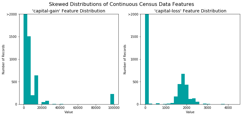
A dataset may sometimes contain at least one feature whose values tend to lie near a single number, but will also have a non-trivial number of vastly larger or smaller values than that single number. Algorithms can be sensitive to such distributions of values and can underperform if the range is not properly normalized. With the census dataset two features fit this description: ‘capital-gain' and 'capital-loss'.
Run the code cell below to plot a histogram of these two features. Note the range of the values present and how they are distributed.
1 | # Split the data into features and target label |
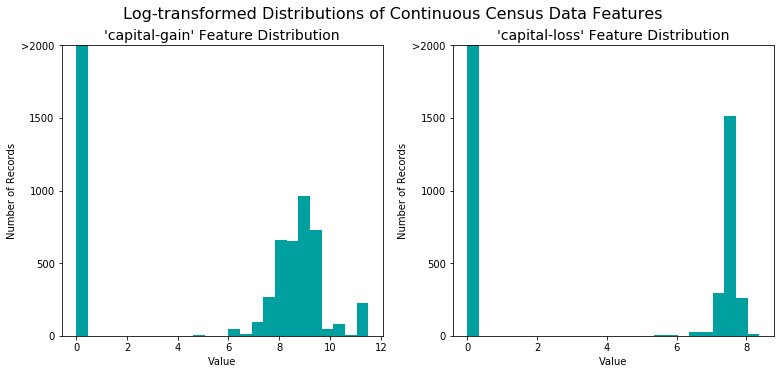
For highly-skewed feature distributions such as 'capital-gain' and 'capital-loss', it is common practice to apply a logarithmic transformation on the data so that the very large and very small values do not negatively affect the performance of a learning algorithm. Using a logarithmic transformation significantly reduces the range of values caused by outliers. Care must be taken when applying this transformation however: The logarithm of 0 is undefined, so we must translate the values by a small amount above 0 to apply the the logarithm successfully.
Run the code cell below to perform a transformation on the data and visualize the results. Again, note the range of values and how they are distributed.
1 | # Log-transform the skewed features |
Normalizing Numerical Features
In addition to performing transformations on features that are highly skewed, it is often good practice to perform some type of scaling on numerical features. Applying a scaling to the data does not change the shape of each feature’s distribution (such as 'capital-gain' or 'capital-loss' above); however, normalization ensures that each feature is treated equally when applying supervised learners. Note that once scaling is applied, observing the data in its raw form will no longer have the same original meaning, as exampled below.
Run the code cell below to normalize each numerical feature. We will use sklearn.preprocessing.MinMaxScaler for this.
1 | # Import sklearn.preprocessing.StandardScaler |
/home/jason/anaconda3/lib/python3.7/site-packages/sklearn/preprocessing/data.py:334: DataConversionWarning: Data with input dtype int64, float64 were all converted to float64 by MinMaxScaler.
return self.partial_fit(X, y)| age | workclass | education_level | education-num | marital-status | occupation | relationship | race | sex | capital-gain | capital-loss | hours-per-week | native-country | |
|---|---|---|---|---|---|---|---|---|---|---|---|---|---|
| 0 | 0.301370 | State-gov | Bachelors | 0.800000 | Never-married | Adm-clerical | Not-in-family | White | Male | 0.667492 | 0.0 | 0.397959 | United-States |
| 1 | 0.452055 | Self-emp-not-inc | Bachelors | 0.800000 | Married-civ-spouse | Exec-managerial | Husband | White | Male | 0.000000 | 0.0 | 0.122449 | United-States |
| 2 | 0.287671 | Private | HS-grad | 0.533333 | Divorced | Handlers-cleaners | Not-in-family | White | Male | 0.000000 | 0.0 | 0.397959 | United-States |
| 3 | 0.493151 | Private | 11th | 0.400000 | Married-civ-spouse | Handlers-cleaners | Husband | Black | Male | 0.000000 | 0.0 | 0.397959 | United-States |
| 4 | 0.150685 | Private | Bachelors | 0.800000 | Married-civ-spouse | Prof-specialty | Wife | Black | Female | 0.000000 | 0.0 | 0.397959 | Cuba |
Implementation: Data Preprocessing
From the table in Exploring the Data above, we can see there are several features for each record that are non-numeric. Typically, learning algorithms expect input to be numeric, which requires that non-numeric features (called categorical variables) be converted. One popular way to convert categorical variables is by using the one-hot encoding scheme. One-hot encoding creates a “dummy” variable for each possible category of each non-numeric feature. For example, assume someFeature has three possible entries: A, B, or C. We then encode this feature into someFeature_A, someFeature_B and someFeature_C.
| someFeature | someFeature_A | someFeature_B | someFeature_C | ||
|---|---|---|---|---|---|
| 0 | B | 0 | 1 | 0 | |
| 1 | C | —-> one-hot encode —-> | 0 | 0 | 1 |
| 2 | A | 1 | 0 | 0 |
Additionally, as with the non-numeric features, we need to convert the non-numeric target label, 'income' to numerical values for the learning algorithm to work. Since there are only two possible categories for this label (“<=50K” and “>50K”), we can avoid using one-hot encoding and simply encode these two categories as 0 and 1, respectively. In code cell below, you will need to implement the following:
- Use
pandas.get_dummies()to perform one-hot encoding on the'features_log_minmax_transform'data. - Convert the target label
'income_raw'to numerical entries.- Set records with “<=50K” to
0and records with “>50K” to1.
- Set records with “<=50K” to
1 | # TODO: One-hot encode the 'features_log_minmax_transform' data using pandas.get_dummies() |
103 total features after one-hot encoding.Shuffle and Split Data
Now all categorical variables have been converted into numerical features, and all numerical features have been normalized. As always, we will now split the data (both features and their labels) into training and test sets. 80% of the data will be used for training and 20% for testing.
Run the code cell below to perform this split.
1 | # Import train_test_split |
Training set has 36177 samples.
Testing set has 9045 samples.
Evaluating Model Performance
In this section, we will investigate four different algorithms, and determine which is best at modeling the data. Three of these algorithms will be supervised learners of your choice, and the fourth algorithm is known as a naive predictor.
Metrics and the Naive Predictor
CharityML, equipped with their research, knows individuals that make more than $50,000 are most likely to donate to their charity. Because of this, CharityML is particularly interested in predicting who makes more than $50,000 accurately. It would seem that using accuracy as a metric for evaluating a particular model’s performace would be appropriate. Additionally, identifying someone that does not make more than $50,000 as someone who does would be detrimental to CharityML, since they are looking to find individuals willing to donate. Therefore, a model’s ability to precisely predict those that make more than $50,000 is more important than the model’s ability to recall those individuals. We can use F-beta score as a metric that considers both precision and recall:
$$ F_{\beta} = (1 + \beta^2) \cdot \frac{precision \cdot recall}{\left( \beta^2 \cdot precision \right) + recall} $$
In particular, when $\beta = 0.5$, more emphasis is placed on precision. This is called the F$_{0.5}$ score (or F-score for simplicity).
Looking at the distribution of classes (those who make at most $50,000, and those who make more), it’s clear most individuals do not make more than $50,000. This can greatly affect accuracy, since we could simply say *”this person does not make more than $50,000”* and generally be right, without ever looking at the data! Making such a statement would be called naive, since we have not considered any information to substantiate the claim. It is always important to consider the naive prediction for your data, to help establish a benchmark for whether a model is performing well. That been said, using that prediction would be pointless: If we predicted all people made less than $50,000, CharityML would identify no one as donors.
Note: Recap of accuracy, precision, recall
** Accuracy ** measures how often the classifier makes the correct prediction. It’s the ratio of the number of correct predictions to the total number of predictions (the number of test data points).
** Precision ** tells us what proportion of messages we classified as spam, actually were spam.
It is a ratio of true positives(words classified as spam, and which are actually spam) to all positives(all words classified as spam, irrespective of whether that was the correct classificatio), in other words it is the ratio of
[True Positives/(True Positives + False Positives)]
** Recall(sensitivity)** tells us what proportion of messages that actually were spam were classified by us as spam.
It is a ratio of true positives(words classified as spam, and which are actually spam) to all the words that were actually spam, in other words it is the ratio of
[True Positives/(True Positives + False Negatives)]
For classification problems that are skewed in their classification distributions like in our case, for example if we had a 100 text messages and only 2 were spam and the rest 98 weren’t, accuracy by itself is not a very good metric. We could classify 90 messages as not spam(including the 2 that were spam but we classify them as not spam, hence they would be false negatives) and 10 as spam(all 10 false positives) and still get a reasonably good accuracy score. For such cases, precision and recall come in very handy. These two metrics can be combined to get the F1 score, which is weighted average(harmonic mean) of the precision and recall scores. This score can range from 0 to 1, with 1 being the best possible F1 score(we take the harmonic mean as we are dealing with ratios).
Question 1 - Naive Predictor Performace
- If we chose a model that always predicted an individual made more than $50,000, what would that model’s accuracy and F-score be on this dataset? You must use the code cell below and assign your results to
'accuracy'and'fscore'to be used later.
** Please note ** that the the purpose of generating a naive predictor is simply to show what a base model without any intelligence would look like. In the real world, ideally your base model would be either the results of a previous model or could be based on a research paper upon which you are looking to improve. When there is no benchmark model set, getting a result better than random choice is a place you could start from.
** HINT: **
- When we have a model that always predicts ‘1’ (i.e. the individual makes more than 50k) then our model will have no True Negatives(TN) or False Negatives(FN) as we are not making any negative(‘0’ value) predictions. Therefore our Accuracy in this case becomes the same as our Precision(True Positives/(True Positives + False Positives)) as every prediction that we have made with value ‘1’ that should have ‘0’ becomes a False Positive; therefore our denominator in this case is the total number of records we have in total.
- Our Recall score(True Positives/(True Positives + False Negatives)) in this setting becomes 1 as we have no False Negatives.
1 | TP = np.sum(income)# Counting the ones as this is the naive case. Note that 'income' is the 'income_raw' data |
Naive Predictor: [Accuracy score: 0.2478, F-score: 0.2917]Supervised Learning Models
The following are some of the supervised learning models that are currently available in scikit-learn that you may choose from:
- Gaussian Naive Bayes (GaussianNB)
- Decision Trees
- Ensemble Methods (Bagging, AdaBoost, Random Forest, Gradient Boosting)
- K-Nearest Neighbors (KNeighbors)
- Stochastic Gradient Descent Classifier (SGDC)
- Support Vector Machines (SVM)
- Logistic Regression
Question 2 - Model Application
List three of the supervised learning models above that are appropriate for this problem that you will test on the census data. For each model chosen
- Describe one real-world application in industry where the model can be applied.
- What are the strengths of the model; when does it perform well?
- What are the weaknesses of the model; when does it perform poorly?
- What makes this model a good candidate for the problem, given what you know about the data?
** HINT: **
Structure your answer in the same format as above^, with 4 parts for each of the three models you pick. Please include references with your answer.
*Answer: *
1. Logistic Regression
1) It can be used in banking system to determine whether a customer will default or not.
2) When the targeted is a dummy variable this model can perform well. It’s highly interpretable and very efficient.
3) It is not suitable for non-linear problems and it is relatively perform worse than other complex methods.
4) In this problem we want to estimate the dummy which are people who have salary over or below 50k. This model is exactly suitable for this situation.
2. Ensemble Methods (Random Forest)
1) It can be used to determine span e-mails or classify user’s profile.
2) It performs better than many other simple models and not likely to be overfitting. It suits non-linear problems.
3) It is not suitable for linear problems, it is hard to interpret, and it requires high computational power.
4) In this problem we have a classification problem and ensemble methods can give us a good model.
3.Support Vector Machines (SVM)
1) It can also be used for classification problems like whether a customer will default or not.
2) SVM is effective in high dimensional spaces and fast.
3) Not suitable for large dataset.
4) In our problem, we have many dimensions, SVM might perform good.
Implementation - Creating a Training and Predicting Pipeline
To properly evaluate the performance of each model you’ve chosen, it’s important that you create a training and predicting pipeline that allows you to quickly and effectively train models using various sizes of training data and perform predictions on the testing data. Your implementation here will be used in the following section.
In the code block below, you will need to implement the following:
- Import
fbeta_scoreandaccuracy_scorefromsklearn.metrics. - Fit the learner to the sampled training data and record the training time.
- Perform predictions on the test data
X_test, and also on the first 300 training pointsX_train[:300].- Record the total prediction time.
- Calculate the accuracy score for both the training subset and testing set.
- Calculate the F-score for both the training subset and testing set.
- Make sure that you set the
betaparameter!
- Make sure that you set the
1 | # TODO: Import two metrics from sklearn - fbeta_score and accuracy_score |
Implementation: Initial Model Evaluation
In the code cell, you will need to implement the following:
- Import the three supervised learning models you’ve discussed in the previous section.
- Initialize the three models and store them in
'clf_A','clf_B', and'clf_C'.- Use a
'random_state'for each model you use, if provided. - Note: Use the default settings for each model — you will tune one specific model in a later section.
- Use a
- Calculate the number of records equal to 1%, 10%, and 100% of the training data.
- Store those values in
'samples_1','samples_10', and'samples_100'respectively.
- Store those values in
Note: Depending on which algorithms you chose, the following implementation may take some time to run!
1 | # TODO: Import the three supervised learning models from sklearn |
LogisticRegression trained on 361 samples.
LogisticRegression trained on 3617 samples.
LogisticRegression trained on 36177 samples.
RandomForestClassifier trained on 361 samples.
RandomForestClassifier trained on 3617 samples.
RandomForestClassifier trained on 36177 samples.
SVC trained on 361 samples.
SVC trained on 3617 samples.
SVC trained on 36177 samples.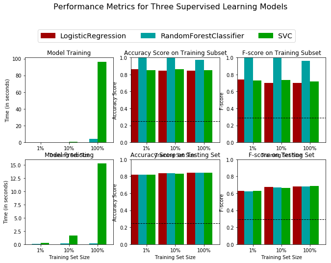
Improving Results
In this final section, you will choose from the three supervised learning models the best model to use on the student data. You will then perform a grid search optimization for the model over the entire training set (X_train and y_train) by tuning at least one parameter to improve upon the untuned model’s F-score.
Question 3 - Choosing the Best Model
- Based on the evaluation you performed earlier, in one to two paragraphs, explain to CharityML which of the three models you believe to be most appropriate for the task of identifying individuals that make more than $50,000.
** HINT: **
Look at the graph at the bottom left from the cell above(the visualization created by vs.evaluate(results, accuracy, fscore)) and check the F score for the testing set when 100% of the training set is used. Which model has the highest score? Your answer should include discussion of the:
- metrics - F score on the testing when 100% of the training data is used,
- prediction/training time
- the algorithm’s suitability for the data.
*Answer: *
The Logistic Regression model is the best model in this situation.
When 100% of the training data is used, the Logistic Regression model has the second highest F-score on testing set with only very slightly difference compared with the best model (SVM). However, it has the lowest training and prediction times, which is faster than the third(best) model quite a lot. Therefore it is wise to choose Logistic Regression model. Actually, Logistic Regression model is very suitable for this data because the targeted variable is a dummy.
Question 4 - Describing the Model in Layman’s Terms
- In one to two paragraphs, explain to CharityML, in layman’s terms, how the final model chosen is supposed to work. Be sure that you are describing the major qualities of the model, such as how the model is trained and how the model makes a prediction. Avoid using advanced mathematical jargon, such as describing equations.
** HINT: **
When explaining your model, if using external resources please include all citations.
*Answer: *
The logistic regression model will create a linear boundary cutting the data points, which can classify whether people have high income or not. It estimates the probability of a person belongs to high income group or low income group based on the change of explaining variables. Logistic regression uses the natural logarithm function to find the relationship between the variables and uses test data to find the coefficients. The function can then predict the future results using these coefficients in the logistic equation.[1] Therefore, this model can split our dataset successfully.

It can be seen in th graph, different from linear model, logistic model is a non-linear function with probability between 0 to 1.
[1] Wikipedia. (2020). Logistic Regression. [online] Available at: https://simple.wikipedia.org/wiki/Logistic_Regression [Accessed 13 Jan. 2020].
Implementation: Model Tuning
Fine tune the chosen model. Use grid search (GridSearchCV) with at least one important parameter tuned with at least 3 different values. You will need to use the entire training set for this. In the code cell below, you will need to implement the following:
- Import
sklearn.grid_search.GridSearchCVandsklearn.metrics.make_scorer. - Initialize the classifier you’ve chosen and store it in
clf.- Set a
random_stateif one is available to the same state you set before.
- Set a
- Create a dictionary of parameters you wish to tune for the chosen model.
- Example:
parameters = {'parameter' : [list of values]}. - Note: Avoid tuning the
max_featuresparameter of your learner if that parameter is available!
- Example:
- Use
make_scorerto create anfbeta_scorescoring object (with $\beta = 0.5$). - Perform grid search on the classifier
clfusing the'scorer', and store it ingrid_obj. - Fit the grid search object to the training data (
X_train,y_train), and store it ingrid_fit.
Note: Depending on the algorithm chosen and the parameter list, the following implementation may take some time to run!
1 | # TODO: Import 'GridSearchCV', 'make_scorer', and any other necessary libraries |
Unoptimized model
------
Accuracy score on testing data: 0.8419
F-score on testing data: 0.6832

Optimized Model
------
Final accuracy score on the testing data: 0.8418
Final F-score on the testing data: 0.6829
Question 5 - Final Model Evaluation
- What is your optimized model’s accuracy and F-score on the testing data?
- Are these scores better or worse than the unoptimized model?
- How do the results from your optimized model compare to the naive predictor benchmarks you found earlier in Question 1?_
Note: Fill in the table below with your results, and then provide discussion in the Answer box.
Results:
| Metric | Unoptimized Model | Optimized Model |
|---|---|---|
| Accuracy Score | 0.8419 | 0.8418 |
| F-score | 0.6832 | 0.6829 |
*Answer: *
The scores for the optimized model is worse than the unoptimized model. The scores for the optimized model improves a lot compared with the naive model.
Feature Importance
An important task when performing supervised learning on a dataset like the census data we study here is determining which features provide the most predictive power. By focusing on the relationship between only a few crucial features and the target label we simplify our understanding of the phenomenon, which is most always a useful thing to do. In the case of this project, that means we wish to identify a small number of features that most strongly predict whether an individual makes at most or more than $50,000.
Choose a scikit-learn classifier (e.g., adaboost, random forests) that has a feature_importance_ attribute, which is a function that ranks the importance of features according to the chosen classifier. In the next python cell fit this classifier to training set and use this attribute to determine the top 5 most important features for the census dataset.
Question 6 - Feature Relevance Observation
When Exploring the Data, it was shown there are thirteen available features for each individual on record in the census data. Of these thirteen records, which five features do you believe to be most important for prediction, and in what order would you rank them and why?
Answer:
education_num: more education might get better jobs
hours-per-week: more working hours more money
age: higher age implies more experience thus more income
marital status: married people might have more incentive to earn more money
sex: it might exists sex discrimination.
Implementation - Extracting Feature Importance
Choose a scikit-learn supervised learning algorithm that has a feature_importance_ attribute availble for it. This attribute is a function that ranks the importance of each feature when making predictions based on the chosen algorithm.
In the code cell below, you will need to implement the following:
- Import a supervised learning model from sklearn if it is different from the three used earlier.
- Train the supervised model on the entire training set.
- Extract the feature importances using
'.feature_importances_'.
1 | # TODO: Import a supervised learning model that has 'feature_importances_' |
/home/jason/anaconda3/lib/python3.7/site-packages/sklearn/model_selection/_split.py:2053: FutureWarning: You should specify a value for 'cv' instead of relying on the default value. The default value will change from 3 to 5 in version 0.22.
  warnings.warn(CV_WARNING, FutureWarning)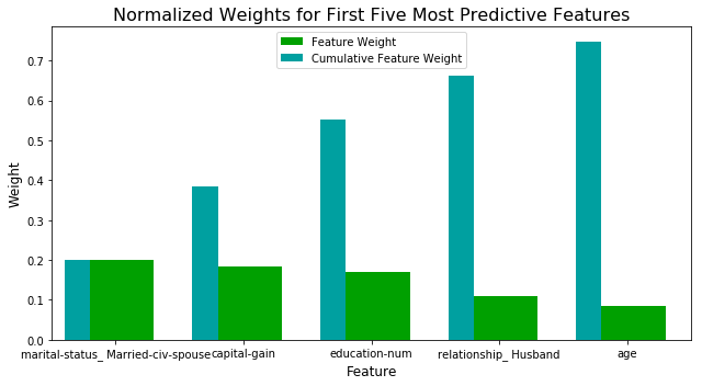
Question 7 - Extracting Feature Importance
Observe the visualization created above which displays the five most relevant features for predicting if an individual makes at most or above $50,000.
- How do these five features compare to the five features you discussed in Question 6?
- If you were close to the same answer, how does this visualization confirm your thoughts?
- If you were not close, why do you think these features are more relevant?
Answer:
Compared with what I thought before, the importance of marital status, ages and years of education are comfirmed by the graph because their weights are high. However, capital-gain and relationship_Husband is not what I predicted.
For capital-gain it might be only whealthy people can have more gain in capital since they have more free money to invest. For relationship, it is kind of overlap with the marital status so the reason is similar as what I explained before that married people are more likely try to earn more money to support the family especially for males.
Feature Selection
How does a model perform if we only use a subset of all the available features in the data? With less features required to train, the expectation is that training and prediction time is much lower — at the cost of performance metrics. From the visualization above, we see that the top five most important features contribute more than half of the importance of all features present in the data. This hints that we can attempt to reduce the feature space and simplify the information required for the model to learn. The code cell below will use the same optimized model you found earlier, and train it on the same training set with only the top five important features.
1 | # Import functionality for cloning a model |
Final Model trained on full data
------
Accuracy on testing data: 0.8418
F-score on testing data: 0.6829

Final Model trained on reduced data
------
Accuracy on testing data: 0.8258
F-score on testing data: 0.6462


/home/jason/anaconda3/lib/python3.7/site-packages/sklearn/utils/validation.py:761: DataConversionWarning: A column-vector y was passed when a 1d array was expected. Please change the shape of y to (n_samples, ), for example using ravel().
  y = column_or_1d(y, warn=True)
Question 8 - Effects of Feature Selection
- How does the final model’s F-score and accuracy score on the reduced data using only five features compare to those same scores when all features are used?
- If training time was a factor, would you consider using the reduced data as your training set?
Answer:
It is actually very close to the full features with slightly lower scores. However since I am using Logistic Regression model, I will not use the reduced data. Because the training time is alreay very short with the full features. The algorithm is very efficient so the room for improvement is quite limited. Therefore it is not wise to sacrifice the model accuracy to save only a few seconds.
Note: Once you have completed all of the code implementations and successfully answered each question above, you may finalize your work by exporting the iPython Notebook as an HTML document. You can do this by using the menu above and navigating to
File -> Download as -> HTML (.html). Include the finished document along with this notebook as your submission.