Deep learning is one of the family members of the machine learning based on artificial neural networks. With the neural networks, images can be classified well.In medical image science deep learning can be used to classify the X-ray images.In this project Chest X-rays are used to classify whether Pneumonia exists. With the model that can classify whether the patient has Pneumonia, doctors can reducetime to read X-ray images. The model will give the possibility of the existence of Pneumonia, which can be used as a auxiliary diagnosis.
1
2
3
4
5
6
7
8
9
10
11
12
13
14
15
16
17
18
19
import matplotlib.pyplot as plt
import torch
from torchvision import datasets,transforms, models
from collections import OrderedDict
import json
import shutil
import numpy as np
import pandas as pd
import time
from torch import nn
from torch import optim
import seaborn as sns
from PIL import Image
from tqdm import tqdm
import glob
import boto3
import sagemaker
from sagemaker.amazon.amazon_estimator import get_image_uri
import os
Introduction
Deep learning is one of the family members of the machine learning based on artificial neural networks. With the neural networks, images can be classified well.In medical image science deep learning can be used to classify the X-ray images.In this project Chest X-rays are used to classify whether Pneumonia exists. With the model that can classify whether the patient has Pneumonia, doctors can reducetime to read X-ray images. The model will give the possibility of the existence of Pneumonia, which can be used as a auxiliary diagnosis.
The problem is to create a model that can classify the chest x-ray image in termsof whether Pneumonia exists. A deep learning method will be used, and AmazonSageMaker will be utilized. A high level method for SageMaker training will bedeployed in building the model
The dataset is organized into 3 folders (train, test, val) and contains subfolders foreach image category (0/1). 0 represents Normal and 1 represents Pneumonia. Thereare 5,863 X-Ray images (JPEG).
The benchmark model can be found in Kaggle. The best model in Kaggle Kernelsright now has recall ratio 0.98 and precision ratio 0.79. My goal is to get the similarresult based on the same test dataset.
Accuracy ratio, recall ratio and precision ratio can be used to evaluate the modelperformance. In this case recall ratio should be focused on since the number ofFalse Negatives should be as low as possible but accuracy ratio should also be considered. Thus the trade off between recall and precision ratio will be considered.
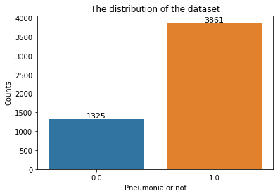
# Then we can see the distribution of our train dataset counts = df_train.pneumonia.value_counts() sns.barplot(x=counts.index, y= counts.values) plt.title('The distribution of the dataset') plt.xlabel('Pneumonia or not') plt.ylabel('Counts') plt.text(0,counts.values[1], '%.0f' % counts.values[1], ha='center', va= 'bottom',fontsize=11) plt.text(1,counts.values[0], '%.0f' % counts.values[0], ha='center', va= 'bottom',fontsize=11)
Text(1, 3861, '3861')
1 2 3 4 5 6 7 8 9 10 11 12 13 14 15 16 17 18 19
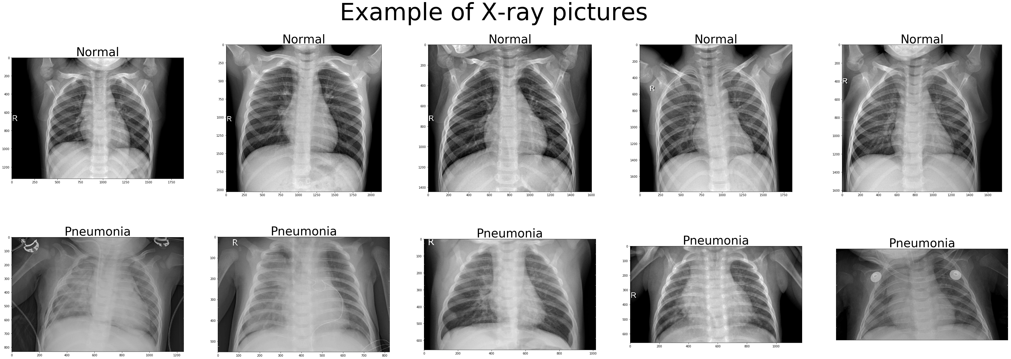
# It is also a good idea to look some examples of the X-ray pictures.
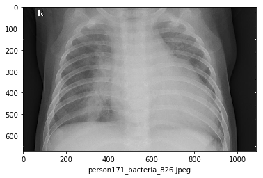
fig, ax = plt.subplots(2,5, figsize=(60,20)) for i in range(1,11): img = Image.open(pic_list[i-1]) if i <= 5: ax[0,i-1].imshow(img, cmap='gray') ax[0,i-1].set_title('Normal',fontsize=40) else: ax[1,i-6].imshow(img, cmap='gray') ax[1,i-6].set_title('Pneumonia',fontsize=40) plt.xticks([]) plt.yticks([]) fig.suptitle('Example of X-ray pictures', fontsize=80) plt.show()
Next we should preprocessing our dataset in order to fit the requirements of the model. In this case, we should create dictionaries such that each file name corresponds to the correct label.
1 2 3 4 5 6 7 8 9
# create annotations for train train_annotations = [] for each in df_train['Pic']: each = each.strip('chest_xray/train/1/') each = each.strip('chest_xray/train/0/') train_annotations.append(each) train_annotations = pd.DataFrame([train_annotations,df_train['pneumonia']]).T train_annotations = dict(train_annotations.values.tolist()) len(train_annotations)
5186
1 2 3 4 5 6 7 8 9
# create annotations for validation valid_annotations = [] for each in df_valid['Pic']: each = each.strip('chest_xray/valid/1/') each = each.strip('chest_xray/valid/0/') valid_annotations.append(each) valid_annotations = pd.DataFrame([valid_annotations,df_valid['pneumonia']]).T valid_annotations = dict(valid_annotations.values.tolist()) len(valid_annotations)
46
1 2 3 4 5 6 7
all_annotations = {}
for key, value in train_annotations.items(): all_annotations[key] = value for key, value in valid_annotations.items(): all_annotations[key] = value len(all_annotations)
5232
1 2 3 4 5 6
classes = list(all_annotations.values())
classes = list(set(classes))
print(classes) print('\nNum of classes:', len(classes))
[0.0, 1.0]
Num of classes: 2
We have 5232 training images and 46 validation images with two classes.
2. Upload the training data to S3
1 2 3 4 5 6
# session and role sess = sagemaker.Session() role = sagemaker.get_execution_role() bucket = sess.default_bucket() container = get_image_uri(boto3.Session().region_name, 'image-classification') print(container)
Training images uploaded
Training list uploaded
validation images uploaded
Validation list uploaded
CPU times: user 36.4 s, sys: 3.31 s, total: 39.7 s
Wall time: 5min 10s
SageMaker Estimator
Then we should set up our model with parameters and hyperparameters.
image_dir = 'chest_xray/test/0' images = [x for x in os.listdir(image_dir) if x[-4:] == 'jpeg'] print(len(images))
234
1
deployed_model.content_type = 'image/jpeg'
1 2 3 4 5 6 7 8 9
index = 233
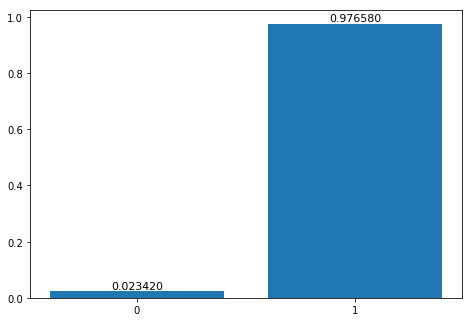
image_path = os.path.join(image_dir, images[index]) with open(image_path, 'rb') as f: b = bytearray(f.read()) result = deployed_model.predict(b) result = json.loads(result) print(result)
# Also try a pneumonia image_dir = 'chest_xray/test/1' images = [x for x in os.listdir(image_dir) if x[-4:] == 'jpeg'] print(len(images))
390
1 2 3 4 5 6 7 8 9
deployed_model.content_type = 'image/jpeg' index = 1 image_path = os.path.join(image_dir, images[index]) with open(image_path, 'rb') as f: b = bytearray(f.read()) result = deployed_model.predict(b) result = json.loads(result) print(result)
The estimates of those examples are correct but we still need to use the remainder test set to calculate the recall and accuracy ratios in order to test our model performence.
Assess the performance
1 2 3 4 5 6 7 8 9 10 11 12 13
# All should be zeros, which means normal image_dir = 'chest_xray/test/0' images = [x for x in os.listdir(image_dir) if x[-4:] == 'jpeg'] deployed_model.content_type = 'image/jpeg' normals = [] for i in range(0,233): index = i image_path = os.path.join(image_dir, images[index]) with open(image_path, 'rb') as f: b = bytearray(f.read()) result = deployed_model.predict(b) result = json.loads(result) normals.append(classes[np.argmax(result)])
# All should be ones, which means pneumonia image_dir = 'chest_xray/test/1' images = [x for x in os.listdir(image_dir) if x[-4:] == 'jpeg'] deployed_model.content_type = 'image/jpeg' pneumonia = [] for i in range(0,389): index = i image_path = os.path.join(image_dir, images[index]) with open(image_path, 'rb') as f: b = bytearray(f.read()) result = deployed_model.predict(b) result = json.loads(result) pneumonia.append(classes[np.argmax(result)])
In this task, recall ratio should be as higher as possible. Based on our model predictions, the recall ratio is nearly 83.5%, which is pretty good. However, if the model will be used in reality the recall ratio should be improved such that number of the miss diagnosis will decrease. Because miss diagnosis will do harm to the patients but false postive can be double checked by the doctor. Next we should improve the recall ratio based on the cutoff values.
Improve the performance of the model
1 2 3 4 5 6 7 8 9 10 11 12 13 14 15 16 17 18 19
cutoff = 0.1# set the cutoff value # All should be zeros, which means normal image_dir = 'chest_xray/test/0' images = [x for x in os.listdir(image_dir) if x[-4:] == 'jpeg'] deployed_model.content_type = 'image/jpeg' normals = [] for i in range(0,233): index = i image_path = os.path.join(image_dir, images[index]) with open(image_path, 'rb') as f: b = bytearray(f.read()) result = deployed_model.predict(b) result = json.loads(result) if result[1] > cutoff: normals.append(1) else: normals.append(0) false_pos = sum(normals) true_neg = len(normals) - false_pos
1
2
3
4
5
6
7
8
9
10
11
12
13
14
15
16
17
18
# All should be ones, which means pneumonia
image_dir = 'chest_xray/test/1'
images = [x for x in os.listdir(image_dir)  if x[-4:] == 'jpeg']
deployed_model.content_type = 'image/jpeg'
pneumonia = []
for i in range(0,389):
    index = i
    image_path = os.path.join(image_dir, images[index])
    with open(image_path, 'rb') as f:
        b = bytearray(f.read())
    result = deployed_model.predict(b)
    result = json.loads(result)
    if result[1] > cutoff:
        pneumonia.append(1)
    else:
        pneumonia.append(0)
true_pos = sum(pneumonia)
false_neg = len(pneumonia) - true_pos
When we set the cutoff value equals 0.2, the recall ratio improves to nearly 96.9%. What is worth to mention is that the precision ratio only decreased a little bit to 88.1%. Therefore, the overall accuracy ratio improves. It is good to choose a relatively lower cutoff value. The usual cutoff value is 0.5 but in this diagnostic problem we should choose relatively lower cutoff value in order to decrease the number of false negatives.
Compared with benchmark model in Kaggle, we have relatively simliar results.
The limitation in this analysis will be the small dataset. This dataset only has nearly 6000 pictures, which is clearly not enough to get an elaborate model. However, the methods and ideas used in this analysis is useful for further analysis when we have more data.