第一个python package -- actupac

一个自己做的精算python包,实现内推和外推利率,并且画出利率曲线。该篇是使用说明和例子。

---

基本介绍

actupac 是一个精算的python包,目前的功能是内推和外推利率,并且画出利率曲线。
代码地址:https://github.com/JasonVictor17/actupac

安装方式

pip install actupac

Collecting actupac
  Downloading https://files.pythonhosted.org/packages/78/6d/100b147d64d2b2653f93818af3da6013f23b53120bdc66e1092133500ff3/actupac-0.1.tar.gz
Building wheels for collected packages: actupac
  Building wheel for actupac (setup.py): started
  Building wheel for actupac (setup.py): finished with status 'done'
  Created wheel for actupac: filename=actupac-0.1-cp37-none-any.whl size=5979 sha256=7eb4984f5edbdd2af0de32a2fb795215bc159ce70f39eb398dead35d5f97950f
  Stored in directory: C:\Users\jasonguo\AppData\Local\pip\Cache\wheels\83\19\8e\472924dcac472b470f64c7e2fdd5553ea1af6857d213253170
Successfully built actupac
Installing collected packages: actupac
Successfully installed actupac-0.1
Note: you may need to restart the kernel to use updated packages.

导入包

from actupac import Interpolation
from actupac import Extrapolation

使用方法

1. 内推

目前有三种方法:piecewise linear, piecewise constant, 以及 cubic spline。 其中 cubic spline 使用两端二次导为零的方法,所以是natural spline。

数据需要存储在csv格式文件中,第一列为年份,第二列为利率即可,不需要列名等。

可以改变的参数是内推点的个数,以下以9个点为例子:

# Read the dataset
sample = Interpolation()
df = sample.read_data('interest.csv')
df.head()

	Years	Yields
0	1	1.129
1	2	1.224
2	3	1.364
3	4	1.540
4	5	1.707

# calculate means and standard deviation and discount rates
print(sample.mean)
print(sample.stdev)
discount = sample.discount_rate()
discount[0:5]

2.3666
0.492





[0.9887734928804884,
 0.9758172050673466,
 0.9599059193497299,
 0.9402589151464628,
 0.9181908613542313]

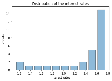
# plot the distribution of the dataset
sample.plot_histogram()

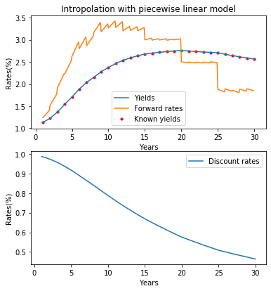
# interpolate with piecewise linear model with 9 interpolated points between each known year
linear = sample.piecewise_linear(9)
print(linear.head())
sample.piecewise_linear_plot()

   Years  Yields        Pt        Ft
0    1.0  1.1290  0.988773  1.234261
1    1.1  1.1385  0.987555  1.253285
2    1.2  1.1480  0.986318  1.272309
3    1.3  1.1575  0.985065  1.291333
4    1.4  1.1670  0.983795  1.310358

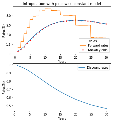
# interpolate with piecewise constant model with 9 interpolated points between each known year
constant = sample.piecewise_constant(9)
print(constant.head())
sample.piecewise_constant_plot()

   Years    Yields        Pt       Ft
0    1.0  1.129000  0.988773  1.31987
1    1.1  1.146273  0.987470  1.31987
2    1.2  1.160667  0.986169  1.31987
3    1.3  1.172846  0.984869  1.31987
4    1.4  1.183286  0.983570  1.31987

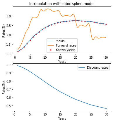
# interpolate with cubic spline (natural spline) model with 9 interpolated points between each known year
cubic = sample.cubic(9)
print(cubic.head())
sample.cubic_plot()

   Years    Yields        Pt        Ft
0    1.0  1.129000  0.988773  1.224226
1    1.1  1.137589  0.987564  1.242089
2    1.2  1.146233  0.986339  1.260836
3    1.3  1.154987  0.985097  1.280690
4    1.4  1.163908  0.983837  1.301870

2. 外推

目前只有 Smith Wilson 方法进行同时外推和内推, 需要手动输入已知数据创建为列表形式即可。 可变参数有三个,n是步长,0.1代表0.1年为一个步长;max_year是外推的最大年份, UFR 是 Ultimate forward rate 可以根据需要改变。

a = list([1,2,3,4,5,10,15,20,30,50])
b = list([3.2870,3.1280,3.2240,3.3680,3.4710,3.9860,4.2070,4.0540,3.4320,2.9310])

# read the data and creat a dataframe
sample2 = Extrapolation(a,b)
sample2.dataframe()

	Years	Yields
0	1.0	3.287
1	2.0	3.128
2	3.0	3.224
3	4.0	3.368
4	5.0	3.471
5	10.0	3.986
6	15.0	4.207
7	20.0	4.054
8	30.0	3.432
9	50.0	2.931

# results 
sample2.Smith_Wilson(n=0.1,max_year=70,UFR=4.2)

	Years	Yields	Discount rates	Forward rates
0	0.0	NaN	1.000000	3.401529
1	0.1	3.395757	0.996610	3.395344
2	0.2	3.392675	0.993238	3.382345
3	0.3	3.387329	0.989889	3.362554
4	0.4	3.379725	0.986572	3.335994
...	...	...	...	...
696	69.6	3.151262	0.111550	4.059759
697	69.7	3.152554	0.111099	4.061264
698	69.8	3.153844	0.110650	4.062754
699	69.9	3.155132	0.110202	4.064228
700	70.0	3.156419	0.109756	NaN

701 rows × 4 columns

# plots
sample2.Smith_Wilson_plot()